
Part 2: Deep Dive into ARIMA
This is a continuation of the Time Series Analysis posts. Here, I will do a deep dive into a time series model called ARIMA, an important smoothing technique used commonly throughout the data science field.
If you have not read part 1 of the series on the general overview of time series, feel free to do so!
VII. ARIMA: Autoregressive Integrated Moving Average
ARIMA stands for Autoregressive Integrated Moving Average. These models aim to describe the correlations in the data with each other. You can use these correlations to predict future values based on past observations and forecast errors. Below are ARIMA terms and definitions you must understand to use ARIMA!
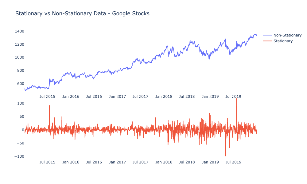
1) Stationarity: One of the most important concepts in time series analysis is stationarity. Stationarity occurs when a shift in time doesn’t change the shape of the distribution of your data. This is in contrast to non-stationary data, where data points have means, variances and covariances that change over time. This means that the data have trends, cycles, random walks or combinations of the three. As a general rule in forecasting, non-stationary data are unpredictable and cannot be modeled.
To run ARIMA, your data needs to be stationary! Again, a time series has stationarity if a shift in time doesn’t cause a change in the shape of the distribution. Basic properties of the distribution like mean, variance, and covariance are constant over time. In layman’s terms, you need to induce stationarity in your data by “removing” systematic component to make the data appear random. This means you must transform your non-stationary dataset to use it with ARIMA. There are two different violations of stationarity, but this is outside the scope of this post. To understand them, please look at this post: understanding stationarity. There are 2 techniques to induce stationarity, and ARIMA fortunately has one way of inducing stationarity by using differencing, which is in the ARIMA equation itself. There are two different tests called the ADF and the KPSS test to check if your data is stationary or not. After running tests, induce stationarity by transforming your data appropriately until it is stationary.
2) Differencing: A transformation of the data that involves subtracting a point at time t with a value at time t-p, where p is a specified lag value. A differencing of one means subtracting the point at time t with the value at t-1 to make the data stationary. The graph below is applying a differencing order of 1 to make data stationary. All of this can be done in many coding libraries and packages.
3) Autoregressive Lag: These are the historical observations of a stationary time series
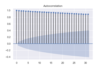
The Autoregressive part in ARIMA is tied to historical aspects of the data. 1 autoregressive lag is the previous data point. Two autoregressive lags refers to two previous data points and so on. This is a critical component to ARIMA, as this will tell you how many of the previous data points you would like to consider when making the next predicted data point. Useful techniques for determining how many autoregressive lags to use in your model are autocorrelation and partial autocorrelation plots.
As an example, see these autocorrelation plots and partial autocorrelation plots below. Because of the drop-off after the second point, this indicates you would use 2 autoregressive lags in your ARIMA model.
4) Moving Average Lags: This is related to historical forecast error windows.
The moving average lags refer to the size of the window you want to use for computing your prediction error when training your model. Two moving average lags means you are using the average error of the previous two data points to help correct the predictions on the data point you are predicting next! For the moving average lags, you specify how big your window size will be. These window sizes will contribute to how many data point errors you want to use for your next prediction. Again, it is useful to determine how many lags you use with autocorrelation and partial autocorrelation plots. For more in-depth analysis of determining autoregressive lags and moving average lags, please take a look at this post about understanding lags.
5) Lag Order: This tells us how many periods back we go. For example, lag order 1 means we use the previous observation as part of the forecast equation.
VIII. Tuning ARIMA and general equation
Now that you know general definitions and terms, I will talk about how these definitions tie into the ARIMA equation itself. Below is the general makeup of an ARIMA model, along with the terms used for calibrating and tuning the model. Each parameter will change the calculations done in the model.
Below are the general parameters of ARIMA:
ARIMA(p, d, q) ~ Autoregressive Integrated Moving Average(AR, I, MA)
p – order of the autoregressive lags (AR Part)
d – order of differencing (Integration Part, I)
q – order of the moving average lags (MA Part)
Below is the general formula for ARIMA that shows how the parameters are used. I will break down each parameter and how they fit into the equation.

1) p – order of the autoregressive lags (AR Part)
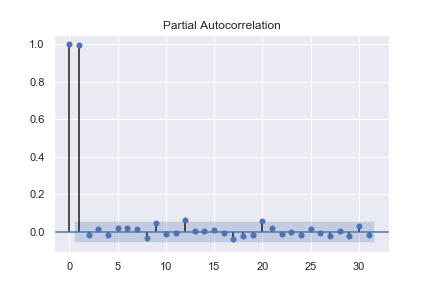
When p=2 and everything else is 0 – ARIMA(2,0,0), you are using the 2 previous data points to contribute to your final prediction. This can be noted in the equation below and is a subset of the entire ARIMA equation.
![]()
The equation gives you a forecast at a particular time if you use p to the order of 2 autoregressive lags. It uses the previous 2 data points and the level at that point in time to make the prediction. For example, the red values below are used to forecast the next point, which would be the first data point on the green line.
2) d – order of differencing (Integration Part, I)
The next parameter in ARIMA is the d parameter, which also the differencing part or integration part. As mentioned earlier, you need to difference your data to make it stationary. When you have non-stationary data, ARIMA can help apply differencing until your data is stationary. The d term in the ARIMA model does this differencing for you. When you apply d=1, you are doing first order differencing. That just means you are differencing once. If you apply d=2, you difference twice. You only want to difference enough to where the data is finally stationary. As I mentioned before, you can check if your data is stationary using the ADF and the KPSS tests. Here are the equations for differencing below. Notice that third, fourth to the nth order differencing can be applied.

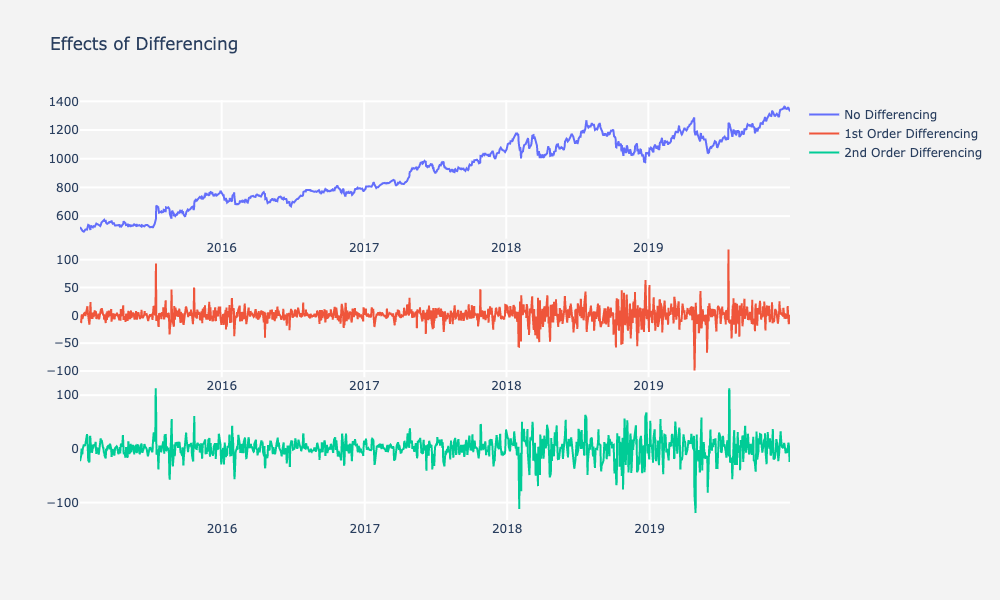
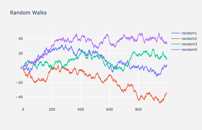
When you apply first order differencing and don’t make any changes to the autoregressive lags or moving average, it is ARIMA(0,1,0), also called a random walk. This means your model is going to generate forecasts without taking into consideration previous data points. Forecasts will be randomly generated.
3) q – order of the moving average lags (MA Part)
Finally, we will talk about the q term. The q term is the moving average part and is applied when you want to look at your prediction error. You will use this error as input for your final forecast at time t. This will be relevant when you are training the data. You can use this parameter to correct some of the mistakes you made in your previous prediction to use for a new prediction. Below is the equation used on the error terms and is the last portion of the general ARIMA equation above:
![]()
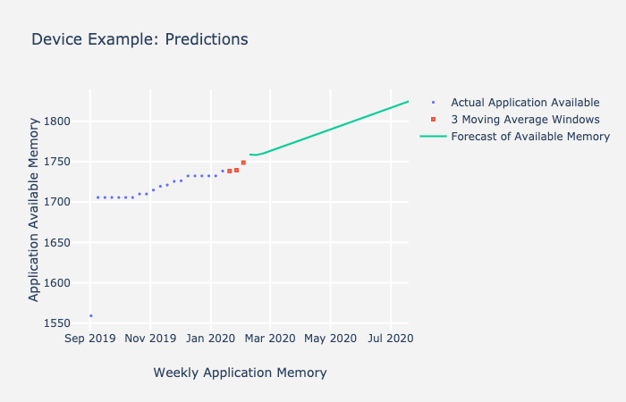
As you can see below, with ARIMA(0,0,3), the three red data points indicate the window size you will use to help make a prediction on the next point. The next forecasted point from the three red points would be the first data point on the green line.
IX. Measuring if Forecast is good or not
1) Train/Test Splits
Now that you know all the components of ARIMA, I will talk about how to make sure your forecasts are good. When you are training a model, you need to split your data into train and test sets. This is so you can evaluate the test set, as this set of values is not trained during model fit. As opposed to other classical machine learning techniques, in which you can split your data randomly, a time series must be a sequential train-test split. Below is an example of a typical train-test split.
2) Model Forecast Error
After you have finished training your model, you need to know how far your predictions are from the actual values. That is where you introduce error metrics. For the predictions on the test set, you can calculate how far off your predictions were from the actual values using various error metrics. Your goal when making a forecast is to reduce this error as much as possible. This is important as it will tell you how good the forecast is. Additionally, knowing your forecasting error will also help you tune your parameters on the ARIMA model should you want to make changes to the model.
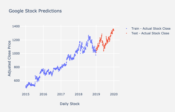
The metrics we generally recommend for time series is mean absolute error and mean absolute percentage error. Mean absolute error (MAE) is a single number, and it tells you on average how far your predictions are from the actual values. Mean average percentage error (MAPE) is another metrics we use, and it is the mean average error expressed as a percentage. This will tell you how “accurate” your model is. The equations for MAE and MAPE are below as well as a plot of Google stock predictions on a train-test split. You can calculate the error on the predictions using the equations below. Notice that you will use the forecasts on the purple line and the red data points to help calculate MAE and MAPE for your test set.


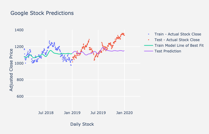
In the example plot above, the line represents your model fit and predictions while the dots represent the actual data. To get the mean absolute error at each time point, you subtract the actual data from the prediction (the points represented as a line in this graph) to get the error. You sum those up and divide by the total number of points. For the forecast on the test set here, the mean absolute error was $72.35, which means on average, each prediction was off by around $72.35. Additionally, the mean absolute percentage error is 5.89%, which tells us that the overall “accuracy” of the model is around 94.11%.
Overview of Steps for tuning ARIMA
Now that you know all of the steps in detail, below I will overview how you want to think about each parameter and steps you would take to train your ARIMA model.
1) Identify the order of differencing, d, using stationarity tests.
2) Identify the order of the autoregression term, p, using ACF plots as rubrics.
3) Identify order of the moving average term, q, using ACF plots as rubrics.
4) Optimize models to minimize error on test data using mean absolute error and mean absolute percentage error after doing a train-test split.
X. Multivariate Forecasting: A Brief Glimpse
Now that you know the basics of tuning ARIMA, I want to mention one more interesting topic. Everything detailed above was in concern of forecasting on one variable. This is called univariate time series. Another important concept arises when you want to predict more than one variable. This is called multivariate forecasting. This will be an important concept that I talk about in Part 3 of the blog series about time series, where I introduce a Cisco use case.
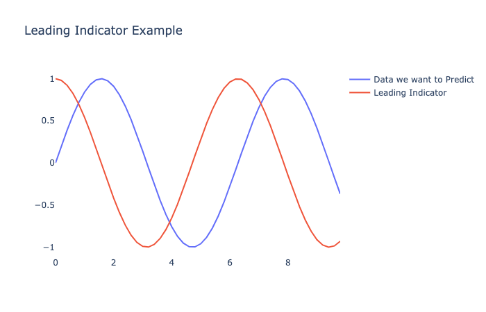
Why would you want to introduce more variables into a time series? There might be a chance that other variables in your dataset might help explain or help predict future values of your target variable. We call these leading indicators. A leading indicator gives a signal after the trend has started and is telling you to pay attention!
For example, let’s say you own an ice cream shop and it is summertime. PG&E cuts off your electricity. You can probably predict that in the future, ice cream sales will go down. You have no electricity to store and make your ice cream in the sweltering heat. The turning off and turning on of electrical power would be a great example of a leading indicator. You can use this indicator to supplement the forecasting of your sales in the future.
There are plenty of Multivariate ARIMA variations, including ARIMAX, SARIMAX, and Vector Autoregression (VAR). I will talk about ARIMAX briefly in the next post.
I hope you enjoyed part 2 of the time series blogs detailing ARIMA and its components! In part 3 of the series, I will talk about a Cisco use case involving predicting memory allocation on Cisco devices.
What is your experience with ARIMA? What is your favorite way to implement it? Let me know in the comments!


