
In part one of this series we covered the internals of HDDs, in part two we went over the internals of SSD, In part three we continue reviewing storage concepts to refresh or learn the right lingo.
Lets start by understanding “Redundant Array of Independent Disks” (RAID). There are RAID levels like RAID0 and RAID1 that are easily to understand and others like RAID5 and RAID6, which many sysadmins misunderstand.
Redundant Array of Independent Disks (RAID)
In the past RAID was also referred as a “Redundant Array of Inexpensive Disks”. At the end of the day, we are talking about a redundant array of disks.
For the purpose of this review we are going to concentrate in the most common RAIDs:
- RAID Level 0
- RAID Level 1
- RAID Level 4 (to clarify concept)
- RAID Level 5
- RAID Level 6
- RAID-DP (to clarify concept)
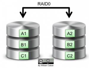
RAID Level 0
RAID Level 0, also known as “stripe” or “striping” split the data across two or more disks. Provides great write performance but there is no data protection. If one of the disks fails, all the data is lost.
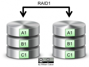
RAID Level 1
RAID Level 1, also known as “mirror” or “mirroring” replicates all the data to across two disks increasing data protection and reliability. When a disk failure occurs, all data is still available from the other disk. Great read performance but has a write performance impact. The effective storage capacity becomes ½ of the total disks capacity.
RAID Level 4 vs RAID Level 5
There is a common misconception between these two so lets cover both at the same time and understand the difference. RAID4 and RAID5 have a minimum of three disks requirement. Both have the equivalent of a minimum of two data disk and one parity disk. Both support a single drive failure. So, what’s the difference?
RAID Level 4 stripe data across at least two data disk and has a dedicated parity disk.
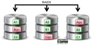
RAID Level 5 stripe data and parity across all available disks using the equivalent space of one disk for parity. Again, the parity is distributed across the available disks.
It is easier to visualize the differences between the two using the following diagrams.
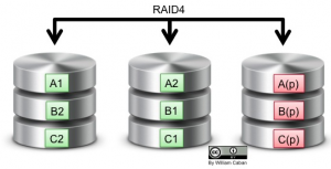
The disadvantage with RAID4 is that the dedicated parity disk end up receiving huge amount of writes, equivalent to all the writes to the array, causing frequent failures to the mechanical components of the parity disk.
With RAID5 we stripe data and parity so we don’t end up stressing a single disk drive. RAID5 is ideal for general workloads since it provides a good balance between protection and performance. The drawback of having a striped parity is that a disk failure will impact the performance for the whole array.
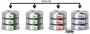
RAID Level 6 vs RAID-DP
Just like what happen with RAID Level 4, there is a common misconception about RAID6. There are no dedicated parity disks in RAID6. Now, there is the standard RAID6 and then there is the NetApp “RAID6” RAID-DP implementation. Both have a minimum requirement of four disks, both can sustain up to two drive failures without data loss.
With RAID6 data and parity are striped among all the available disks using the equivalent space of two disks for parity.
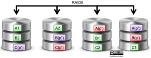
For historical reasons, NetApp RAID-DP does uses two dedicated parity disks. There is an interesting twist with the second parity, even when it is referred as “double parity”, in fact, the second parity is a “diagonal parity”. I’m not going into details but here is a diagram to help illustrate the differences between RAID6 and RAID-DP.
With support for up to two disk failures, in general, RAID6 provides excellent fault-tolerance and performance for mission critical applications. Depending on the implementation, if not handled correctly, RAID6 might cause overhead to the controllers during disk parity calculations.
RAID (Write) Penalty
When we talk about RAID we got to talk about RAID write penalty. This is part of the lingo we now need to understand. Every time we write or read data from a disk we are doing I/O operations. The metrics we use for this performance parameter are IOPS (Input/Output Operations Per Second).
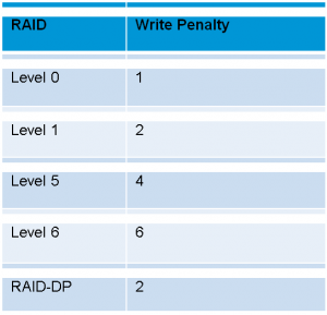
We can’t get this maximum amount of IOPS in a RAID because a parity calculation needs to be done to write data to the disk so that we can recover from a drive failure. These additional operations are the RAID Write Penalty or RAID penalty. So, RAID penalty only comes into play during writes operations. A RAID 0 or stripe has no write penalty associated with it since there is no parity to be calculated. A no RAID penalty is expressed as a RAID Penalty of 1. The following table summarizes the write penalty per RAID level.
Lets understand how the Write Penalty works for RAID 6 and you’ll be able to figure out the others. Lets say we want to change one bit for the striped data. The operations will be something like this:
- I/O#1: Read the striped old_data, XOR with the new_data and obtain the delta_data. Calculate new_parity#1. (We need to read the current data in disk so we can calculate the delta so the write result represents our new_data)
- I/O#2: Read old_parity#1. Calculate delta of old_party#1 and new_partity#1 to obtain delta_parity#1.
- I/O#3: Read old_parity#2. Calculate delta of delta_data + new_partiy#1 + old_parity#2 to obtain delta_parity#2.
- I/O#4: Write delta_data.
- I/O#5: Write delta_parity1
- I/O#6: Write delta_parity2
The order may vary but the operations remain the same. Also, each vendor may implement them differently and as such, they may optimize the operations and end up with more or less IOPS.
From this example you can correlate to the others write penalties. In the case of RAID-DP, they use an NVRAM at the controllers where they do all the calculations and write changes at predefined intervals.
IOPS (Input/Output Operations Per Second)
As you may notice, we are talking about operations not about amount of data, not the amount of bandwidth or the throughput. Here is the first warning: Talking about IOPS without telling you if those are read IOPS, write IOPS and the block size on those operations, does not tell us about the performance of a storage system. It just tells us the amount of operations per second. So, which one is better: 10 write IOPS of 4KB or 2 write IOPS of 10MB?
KB vs KiB
Another differentiation you will see with the lingo of storage guys is the constant distinction between KB vs KiB or MB vs MiB. Basically, when we talk about 1KB = 1,000 Bytes, 1KiB = 1,024 Bytes.
Bandwidth vs Throughput
Quite often you may find system, network and storage administrators using the terms bandwidth and throughput interchangeably. Lets go back to definitions:
- Bandwidth (computing): the peak useful bitrate of a channel
- Throughput (computing): rate of successful message delivery over a communication channel. (for storage this are the IOPS required to complete an operation)
Buffer vs Cache
In storage you will constantly hear about vendors using cache to improve performance for high performance workloads or to use capacity disks in the back, while others increase buffer capacity on their controllers or disks. So, what’s the difference?
- Buffer:
Temporary memory used to store output or input data while it is transferred. (Usually a battery protected memory or disk)
Data is temporarily stored in buffers until enough data is available to pass to the next stage
- Cache:
Temporary memory that transparently stores data so that future requests for that data can be served faster
Area to maintain the most used data (hot data) so any application will first check cache before going to the main storage
Drawbacks
High number of read/write requests fill cache and then it becomes the bottleneck. After cache is filled, additional writes/reads hit directly the regular disks and performance drop to whatever the regular disks can provide.
Write Cache with SSDs or Disk Cache: use SSDs disk to increase performance and protect data in case of power failures but shorten the lifetime of SSDs.
Data Reduction
Data reduction is an umbrella term to refer to multiple techniques used by the industry to optimize the storage utilization. The two common techniques for data reduction are Compression and deduplication. We can find manufacturers with high compression and/or deduplication ratio but at the end, the achievable compression and/or deduplication ratio is dependent on the kind of data. With uncompressed data, like text or raw formats, compression and deduplication have tremendous gain. While for data like videos or jpegs, the achievable compression and deduplication might be minimal. (Well, unless you keep multiple copies of the same videos and jpegs).
IOPS Per Disk Type
Each disk type provides certain amount of IOPS. These IOPS will account towards the amount of raw IOPS a system can provide.
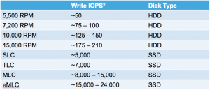
*Write IOPS varies among vendors and disk models
How many disks? How many IOPS?
If we would live in a perfect world without RAID penalty calculating the amount of disk to achieve certain amount of IOPS would be a simple addition, but we have the RAID penalty.
Here are some basic formulas a storage administrator would learn:
- Total Raw IOPS = Disk IOPS * Number of disks
- Functional IOPS = (Raw IOPS * Write%) / (Raid Penalty) + (Raw IOPS * Read %)
How many disks are required to achieve certain number of IOPS?
- Disks Required = ((Read IOPS) + (Write IOPS*Raid Penalty)) / Disk IOPS
Traditionally, we would need to do something like this.
Lets say we want to know how many disks we need to achieve 2000 IOPS for a typical VDI workload that is 80% writes and 20% reads and we want to use 15K RPMs disks (180 IOPS per disk).
Disks Required = ((Raw IOPS * Read%) + ((Raw IOPS * Write%) * Raid Penalty)) / Disk IOPS
[(400) + (1600* Raid Penalty)] / 180 = ??
![]()
Following the math it means that to run this VDI workload we would need 39 disks using RAID5 and 58 disks using RAID6.
Here is where workload characterization comes into play because if we understand the workload behavior, we can use or more cache or larger buffers to reduce the amount of disks. Here is where the UCS Invicta as application acceleration comes into play.
Those are part of the pains and part of the basic lingo we use in storage arrays. In part four we will see how UCS Invicta works and how it simplifies our datacenter.


